NOTE: This introduction is intended for professional astronomers and expert users. For a step-by-step tutorial intended for educators and non-experts, see the Searching for Data How-To Tutorial.

SQL is the Structured Query Language, a standard means of asking for data from databases, and is used to query the Catalog Archive Server (CAS). This page provides a brief overview of SQL. The searching tutorial provides some example queries, with comments, as well as a page of links to more detailed off-site documentation. Examples here will use the sdssQA.

• Database Fundamentals
• Query Fundamentals
• Simple Logical/Mathematical Operations
• Joins: Querying With Multiple Tables
• More Complex Queries: Using distinct, group by, order by, etc.
• Optimizing Queries **IMPORTANT!**
• Searching Tutorial

Database Fundamentals

When performing queries, you must first decide which database you will be using. There are two main databases in the CAS, Target and Best. In the DR1, these databases are actually named TARGDR1 and BESTDR1. The Target database contains all measurements as they were made when objects were targeted for spectroscopy. Best contains the best data and most recent processings for the entire released sky area. The area coverage is almost, but not exactly, the same. By default, queries are made on the Best database. To use a different database, you can use the .. syntax to specify a table in the other database, for instance:

TARGDR1..PhotoObj

If you are using the sdssQA, you can select the server and database using Options->Config, or the areas in the upper right of the query window (shown below).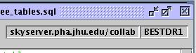

For more details on the differences between Target and Best, please see the data model page.

Each database contains a large number of tables, some of which contain photometric measurements (such as PhotoObj), spectroscopic measurements (such as SpecObj), or information about the observing conditions (Field) or survey geometry(TileBoundary). See the data model page for more details.

In addition to the tables, we have defined Views, which are subsets or combinations of the data stored in the tables. Views are queried the same way Tables are; they exist just to make your life easier. For instance, the view Galaxy can be used to get photometric data on objects we classify as galaxies, without having to specify the classification in your query.

Both the Skyserver and sdssQA interfaces have an Object Browser. This does not let you browse astronomical objects! It shows you all of the available databases, the tables in each database, and the quantities stored in each column of the tables.

Finally, we have created a variety of functions and stored procedures which let you easily perform some common operations. Usually, their names are prefixed by f or sp, like in fPhotoStatus or spGetFiberList. The full list of functions and store procedures is found in the Object Browser. Note that some functions are scalar-valued, meaning that they return a single value, while others (such as the commonly used dbo.fGetNearbyObjEq, are table-valued; they actually return a table of data, and not a single number. This is important when interpreting the returned data and performing joins.

Query Fundamentals

Now that we have an overview of the database structure, how do we actually get data out? You will have to write a query using SQL. The most basic query consists of three parts:

1. A SELECT clause, which specifies the parameters you wish to retrieve;
2. A FROM clause, which specifies the database tables you want to extract the data from;
3. A WHERE clause, which specifies the limitations/predicates you want to place on the extracted data.

The WHERE clause is not necessary if you want to retrieve parameters of all objects in a specified table, but this typically will be an overwhelming amount of data!

Note that the query language is insensitive to splitting the query over many lines. It is also not case sensitive. To make queries more readable, it is common practice to write the distinct query clauses on separate lines. The File->Load Example Queries menu item in the sdssQA window provides a variety of samples, ordered in complexity. For instance, to obtain the list of unique Fields that have been loaded into the database, we use:

SELECT FieldID
FROM Field

You can just copy and paste this (or any other) query into the SQL window of SkyServer, and press submit, or into the sdssQA query window, and press the green arrow button to submit.

If we want to retrieve multiple parameters from the database, we separate them with commas:

SELECT ra,dec 
FROM Galaxy

Of course, the parameters you request must be included in the table(s) you are querying! Now, let's say we want magnitudes of all bright galaxies. We will need to specify a magnitude range to do this:

SELECT u,g,r,i,z
FROM Galaxy
WHERE r<12 and r>0

Here, we have used the WHERE clause to provide a magnitude range. The and operator is used to require that multiple limits be met. This leads us to...

Simple Logical and Mathematical Operators

Not only can we place limits on individual parameters, we can place multiple limits using logical operators, as well as place limits on the results of mathematical operations on multiple parameters. We may also retrieve results that are logical joins of multiple queries. Here we list the logical, comparison, and mathematical operators.

The LOGICAL operators are AND,OR,NOT; they work as follows:

When comparing values, you will use the COMPARISON operators:

In addition to the comparison operators, the special BETWEEN construct is available.
a BETWEEN x AND y is equivalent to a >= x AND a <= y

Similarly,
a NOT BETWEEN x AND y is equivalent to a < x OR a > y

Finally, the MATHEMATICAL operators (both numeric and bitwise) are:

In addition, the usual mathematical and trigonometric functions are available in SQL, such as COS, SIN, TAN, ACOS, etc..

Joins: Querying With Multiple Tables

You may wish to obtain quantities from multiple tables, or place constraints on quantities in one table while obtaining measurements from another. For instance, you may want magnitudes (from PhotoObj) from all objects spectroscopically identified (SpecObj) as galaxies. To perform these types of queries, you must use a join. You can join any two (or more) tables in the databases as long as they have some quantity in common (typically an object or field ID). To actually perform the join, you must have a constraint in the WHERE clause of your query forcing the common quantity to be equal in the two tables.Here is an example, getting the g magnitudes for stars in fields where the PSF fitting worked well:

SELECT s.psfMag_g
FROM Star s, Field f
WHERE s.fieldID = f.fieldID
  and  s.psfMag_g < 20 
  and  f.pspStatus = 2

Notice how we define abbreviations for the table names in the FROM clause; this is not necessary but makes for a lot less typing. Also, you do not have to ask for quantities to be returned from all the tables. You must specify all the tables on which you place constraints (including the join) in the FROM clause, but you can use any subset of these tables in the SELECT. If you use more than two tables, they do not all need to be joined on the same quantity. For instance, this three way join is perfectly acceptable:

SELECT p.objID,f.field,g.run
FROM PhotoObj p, Field f, Segment g
WHERE
  f.fieldid = p.fieldid
  and  f.segmentid = g.segmentid

The type of joins shown above are called inner joins. In the above examples, we only return those objects which are matched between the multiple tables. If we want to include all rows of one of the tables, regardless of whether or not they are matched to another table, we must perform an outer join. One example is to get photometric data for all objects, while getting the spectroscopic data for those objects that have spectroscopy.

In the example below, we perform a left outer join, which means that we will get all entries (regardless of matching) from the table on the left side of the join. In the example below, the join is on P.objID = s.BestObjID; therefore, we will get all photometric (P) objects, with data from the spectroscopy if it exists. If there is no spectroscopic data for an object, we'll still get the photometric measurements but have nulls for the corresponding cpectroscopy.

select P.objID, P.ra, P.dec, S.SpecObjId, S.ra, S.dec
from PhotoObj as P left outer join SpecObjAll as S
on P.objID = s.BestObjID

You can join across more than one table, as long as every pair you are joining has a quantity in common; not all tables need be joined on the same quantity. For example:

SELECT TOP 1000
   g.run,
   f.field,
   p.objID
FROM
   photoObj p, field f, segment g
WHERE
  f.fieldid = p.fieldid
  and  f.segmentid = g.segmentid
  and  f.psfWidth_r > 1.2
  and  p.colc > 400.0

Note how the Field and PhotoObj are joined on the fieldID, while the join between Field and Segment uses segmentID.

When using table valued functions, you must do the join explicitly (rather than using "="). To do this, we use the syntax
SELECT quantities
FROM table1
JOIN table2 on table1.quantity = table2.quantity
WHERE constraints
For instance, in the example below, we use the function dbo.fGetNearbyObjEq to get all objects within a given radius (in this case, 1') of a specified coordinate. This is a table-valued, so it returns a table, containing the ObjIDs and distances of nearby objects. We want to get further photometric parameters on the returned objects, so we must join the output table with PhotoObj.:

SELECT G.objID, GN.distance
FROM Galaxy as G
JOIN dbo.fGetNearbyObjEq(115.,32.5, 1) as GN
  on G.objID = GN.objID 
WHERE (G.flags & dbo.fPhotoFlags('saturated')) = 0

More Complex Queries

SQL provides a number of ways to reorder, group, or otherwise arrange the output of your queries. Some of these options are:

• count: Just tell me how many objects would be returned by my query. Example:

  SELECT count(r) 
  FROM Galaxy
  

• distinct: Return only the unique values of the quantities requested in the SELECT statement. Example:

  SELECT distinct run 
  FROM Field
  

• top: Return only the first n rows of the query results. Example:

  SELECT top 100 r
  FROM Star
  

• order by: Order the output by the specified quantities. Default is ascending order, but you can specify descending as well. You can also order by multiple columns. Example:

  SELECT top 1000 u,g,r
  FROM Star
  order by g,r desc
  

• group by: Group the output by the specified quantities. For instance, you could have all the stars in the output, followed by the galaxies. You could also perform operations on the grouped quantities. You could get the min and max magnitudes for stars and galaxies separately, as shown below:

  SELECT min(r),max(r)
  FROM PhotoPrimary
  group by type
  

  You can use this to count how many of each object type is loaded as primary photometric objects, for instance:

  SELECT count(r)
  FROM PhotoPrimary
  group by type
  

Optimizing Queries

It is easy to construct very complex queries which can take a long time to execute. When writing queries, one can often rewrite them to run faster. This is called optimization.

The first, and most trivial, optimization trick is to use the minimal Table or View for your query. For instance, if all you care about are galaxies, use the Galaxy view in your FROM clause, instead of PhotoObj. We have also created a 'miniature' version of PhotoObjAll, called PhotoTag. This miniature contains all the objects in PhotoObjAll, but only a subset of the measured quantities. Using the PhotoTag table to speed up the query only makes sense if you do NOT want parameters that are only available in the full PhotoObjAll.

It is extremely useful to think about how a database handles queries, rather than trying to write a plain, sequential list of constraints. NOT every query that is syntactically correct will necessarily be efficient; the built-in query optimizer is not perfect! Thus, writing queries such that they use the tricks below can produce significant speed improvements.

Here is a staggering example of the importance of optimization:
Find the positions and magnitudes of photometric objects that have been Targeted for spectroscopy as possible QSOs.

A user's first instinct would be to get the desired objects from the PhotoObj table within the TARGDR1 database (which contains the information, including targeting decisions, for objects when they were targeted (chosen) for spectroscopy). So, this query might look like:

SELECT p.ra, p.dec, p.modelMag_i, p.extinction_i
FROM TARGDR1..PhotoObjAll p
WHERE (p.primtarget & 0x00000002 > 0) or (p.primtarget & 0x00000004 > 0)

That's really simple - all you are doing is checking if the primary target flags (primtarget) are set for the two types of QSO targets. This query can take hours, because a sequential scan of every object in the photometric database is required!

One quick change which makes a difference is to simplify the WHERE clause, to get rid of the or, by masking everything but bits 2,4, and checking if the result is non zero. This changes the WHERE clause to:

WHERE  (primtarget & 0x00000006) > 0

This helps a little, but not much - we are still scanning the entire PhotoObj table. We can make our lives a lot better by realizing that the database developers have anticipated that people will be interested in targetting information, and created a smaller table TargetInfo, that contains only the Targetted objects, which is a small subset of the entire photometric database! Using this table, we can rewrite our query as:

SELECT p.ra, p.dec, p.i, p.extinction_i
FROM TargetInfo t, PhotoObjAll p 
WHERE (t.primtarget & 0x00000006>0)
       and p.objid=t.targetobjid

Note how most of the WHERE clause is performed using the Targetinfo table; the SQL optimizer immediately recognizes that this table is much smaller than PhotoObj, and does this part of the search first. The query now runs in 33 seconds, and returns 32931 rows. That is two orders of magnitude improvement over the initial method!.

Finally, we can recognize that all the quantities of interest are also in the PhotoTag table, which contains all the objects in PhotoObjAll, but not all measured quantities. The query will be:

SELECT p.ra, p.dec, p.ModelMag_i, p.extinction_i
FROM TargetInfo t, PhotoTag p 
WHERE (t.primtarget & 0x00000006>0)
       and p.objid=t.targetobjid

This runs in 18 sec, and returns the same 32931 rows. Another factor of two in speed! Note how PhotoObjTag does not contain the simplified i magnitude, and we must use ModelMag_i instead.

Another of the simplest ways to make queries faster is to first perform a query using only indexed quantities, and then select those parameters from the returned subset of objects. An indexed quantity is one where a look-up table has effectively been calculated, so that the database software does not have to do a time-consuming sequential search through all the objects in the table. For instance, sky coordinates cx,cy,cz are indexed using a Hierarchical Triangular Mesh (HTM). So, you can make a query faster by rewriting it such that it is nested; the inner query grabs the entire row for objects of interest based on the indexed quantities, while the outer query then gets the specific quantities desired.