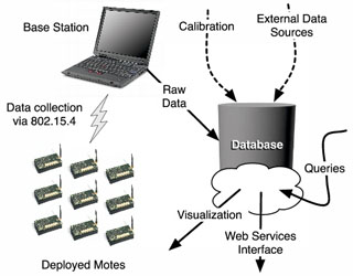
System Architecture

Data Collection Subsystem

Fig.1. Architecture of the end-to-end data collection system

Motes sample data every minute and store them on a circular buffer in their local flash. We use the on-board flash memory so that we can retrieve all observed data even over lossy wireless links -- in contrast to sample-and-collect schemes such as TinyDB which can lose up to 50% of the collected measurements [TPS+05]. Since the mote collects 23KB per day, the MicaZ 512KB flash measurements will be overwritten if not collected within 22 days. In practice, the sensor measurements we downloaded from the motes weekly or at least once every two weeks. To ensure reliable delivery, the base station requests the mote's stored data using a simple sliding window ARQ protocol, and stores the retrieved measurements in the database.

Database

Fig.2. Wireless Sensor Network Database Schema

The database, implemented in Microsoft SQL Server 2005, benefits from the skyserver.sdss.org database we built for Astronomy applications. It inherited a self-documenting framework that uses embedded markup tags in the comments of the DDL scripts to characterize the metadata (units, descriptions, enumerations, etc.) for the database objects, tables, views, stored procedures, and columns. The DDL is parsed a second time, and the metadata information is extracted and inserted into the database itself. A set of stored procedures generate an HTML rendering of the hyperlinked documentation (see Schema Browser on our website.

Data Loading

To date we have loaded 1.6M readings of 3-5 sensors per node, for a total of 6M data points. Raw measurements arrive from the base station as ASCII files in comma-separated-list format. The data are first loaded into a temporary table, where duplicates are removed. The data is next copied into the RawData table, with the \textit{processed} flag set to 0. Converting the raw data to scientifically meaningful values requires a multi-step pipeline performed within the database as a stored procedure. The conversions apply to all $processed = 0$ RawData values. Each produces a Derived measurement and the \textit{RawData.processed} flag is set to 1. The interface boards on some sensors had a loose connection for a while. These RawData measurements are invalid. These intervals are represented in a BadData table, and the corresponding rows in the Derived table are marked with an \textit{isBad=1} flag.

Background weather data from the BWI airport is harvested monthly in CSV format from \verb|wunderground.com| and loaded into the WeatherInfo table. This data includes temperature, precipitation, humidity, pressure and weather events (rain, snow, thunderstorm, etc).

Calibration

We also performed a preliminary check with the soil thermistors and found they are ``relatively'' precise (±0.5°C), yet consistently returned values 1.5$^\circ$C below a NIST approved thermocouple. The 1.5°C bias does not present a large problem because we used the manufacturer's regression technique to convert resistance to temperature. Furthermore, there is 10 kΩ reference resistance connected in series with the moisture sensors on each mote. Since their value directly factors into the estimation of the sensor resistance, the bias is individually measured, recorded in the database, and used during the conversion from raw to derived temperature.

Individual calibration clearly offers us a powerful tool to reduce the measurements' error bar, but how can it be accomplished? The temperature sensors can be calibrated relatively easily as their output (resistance) is only a function of temperature but the moisture sensors require a two-dimensional function that relates resistance to both soil moisture and temperature. The method we used to individually calibrate a Watermark is by taking resistance values at nine points (three moisture contents each at three temperatures), and use these values to calculate individual coefficients to an already published regression form.

Figure 3. Calibration workflow converting raw to derived science dat

Figure 3 illustrates the data flow in the calibration pipeline. This pipeline, implemented within the database, gives the precision and accuracy necessary for sensor-based science.

Data Access and Analysis

The user can specify a window of interest (typically several days), and also a time-step over which the sensor reading are averaged over (a few hours). In another form the users can enter free form SQL for unlimited access to any data item in the database. Outputs can be formatted as HTML rendered tables, CSV files, or XML documents. We also provide a Web Services interface to display the node locations on a map, the values of a particular sensor displayed in color. The time series data can also be displayed in a graphical format, using a .NET web service, calling the same underlying functions or using the built-in SQL Server Reporting Services. This is an area that needs considerably more work -- soil scientists do not want to learn SQL and they often want to see graphical and spatial displays rather than tables of numbers. Beyond better reporting, we plan to use database OLAP and data mining tools.

In addition to analyzing the low level readings looking for unusual cases, ecologists analyze aggregations and averages of the sensor data. We are implementing datacube of the measurements so that spatial and temporal averaging and correlation functions can be displayed more easily and quickly. These aggregates pivot on several dimensions: position on the hillside, depth in the soil, shade vs in the open, etc. This OLAP data cube, using SQL Server Analysis Services will be accessible via the web and web services interface.