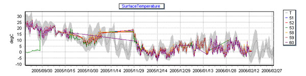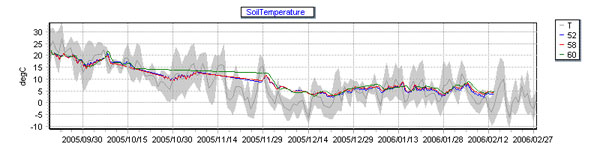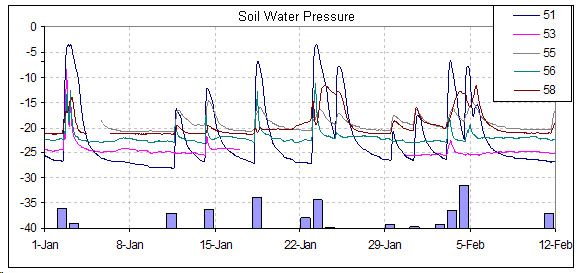
Results

A wireless base station connected to a PC with Internet access resides in an office window facing the deployment. Originally this base station was expected to directly collect samples from the motes. Once the motes were deployed, however, we quickly determined that some motes could not be reliably and consistently reached by our base station. Our temporary solution to this problem was to travel to the perimeter of the deployment site and collect the measurements using a laptop connected to a mote acting as base station.

Ecology Results

Soil moisture data correspond extremely well with precipitation events in the area. The curves reflect cycles of quick wetting and slower drying. During the initial installation, saturated Watermark sensors were placed in the soil surrounded by a saturated slurry. We found that about a week was necessary for the sensor to equilibrate with its surrounding. The shape of the soil water characteristic curve depends on soil type, texture and organic matter content being two important factors [MC04]. Thus, although the curves on Fig 2. reflect typical wetting and drying cycles, they are unique to our field site.

The motes were deliberately placed along a moisture gradient, our system captured spatial heterogeneity of the site. For instance mote 51 (Fig. 2) placed high on the slope showed greater fluctuations then mote 58, which was closer to the stream. We occasionally performed synoptic measurements with Dynamax Thetaprobe sensors to verify our results.

Overall the system reflected the spatiotemporal heterogeneity of the two abiotic factors. Not every sensor worked smoothly, and there were some missing data. However, the differences among the measurements were obvious, and we are confident that these differences reflect real patchiness. Such information will lead to improved surface and groundwater models [Cardell05b], prepare better irrigation plans [MC04] and water resource management. Soil ecologist will be able to better predict where and when the microbial and invertebrate activity occur. This activity is tightly coupled with soil respiration, which is an important, but largely unknown component of the global carbon cycle. Continuous in situ monitoring of these processes will result in better estimates of the contribution of the soil biota to these large scale processes.

Figure 1. Air and soil temperature over a period of ten weeks. Each point represents six hour averages. Tsoil: soil temperature at 10 cm depth; Tsurf: air temperature at soil surface; Thi and Tlow: maximum and minimum temperatures, respectively, for the Baltimore Metropolitan Area.

Figure 2. Soil moisture readings over six weeks recorded by six nodes. Each point represents six hour averages. Bars on the bottom indicate precipitation events in the Baltimore Metropolitan Area. Highest column (Feb 5) corresponds to 25.4 mm rain.

Discussion

We learned what many others have reported, reprogramming and monitoring are essential for managing network deployments \cite{deluge}. Reprogramming allows changing the network's behavior once a fault has been detected, in-situ monitoring allows fault detection and diagnosis [TC05].

Contrary to the promise of cheap WSNs, sensor nodes are still expensive. We estimated the cost per mote including the main unit, sensor board, custom sensors, enclosure, and the time required to implement, debug and maintain the code to be around $1,000, equivalent to the price of a mid-range PC! Calibrating each of the sensors costs more than the sensors themselves -- and is not novice task. The equipment cost will eventually be reduced through economies of scale, but there is clearly a need for standardized connectors for connecting external sensors and in general a need to minimize the amount of custom hardware work necessary to deploy a sensor network. Unfortunately, sensor and mote vendors seem to want proprietary interfaces to encourage lock-in.

We also found that low-level programming is (still) a necessary and challenging task when building sensor networks. Not only did we have to write low-level device drivers for the soil temperature and humidity sensors, but also for power control, as well as for calibration procedures. Moreover, using acquisitional processors such as TinyDB [MFHH04], was not an option in our case given the requirement to collect all the data. Finally, there is need for network design and deployment tools that instruct scientists where to place gateways and sensor relay points. These tools will replace the current trial and error, labor-intensive process of manual topology adjustments that disturbs the deployment area.

Remarks

While the computer science community has focused attention on routing algorithms, self-organization, and in network processing among other things, environmental monitoring applications require quite different emphasis: reliable delivery of the majority (if not all) of the data and metadata to the scientists, high quality measurements, and reliable operation over long deployment cycles. We believe that focusing on these set of problems will lead to interesting new avenues in WSN research.